Martin E Flashman
flashman@humboldt.edu
Humboldt State University
Dept. of Mathematics
Arcata, CA 955521.
Using Probability to Understand Calculus
Though probability is presented briefly in calculus books in a single section or two, no current calculus text has treated probability as an interpretation or application that presents the calculus concepts consistently along with those of probability.
This work is connected toThe Sensible Calculus Program.
Below are several examples illustrating how probability concepts can work as interpretations compared with the more traditional interpretations.
| Motion [Geometry] Interpretation | Probability Interpretation | |
| 0.Generic Example(s) and Precalculus concepts: Functions and Rates. | Motion of an object.
Position functions. Constant velocity. Average velocity. |
Measurement of a random variable.
(Cumulative) Distribution functions. Uniform distribution functions. Average Probability Density. |
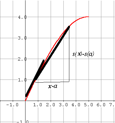
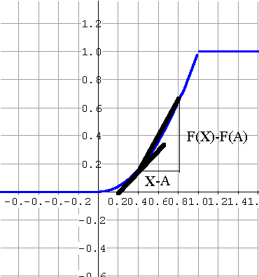
| I. The Derivative. | Position functions determine velocity functions as limits of average velocity. | Distribution functions determine density functions as limits of average probability density. |
| II.Applications of continuity and derivative analysis. | Midway point, Maximum velocity, Mean velocity. | The Median, Mode, and Mean. |
| III. Differential Equations. | Initial Value Problems | Boundary Value Problems |
| IV.The Integral. | Velocity determines position functions.
The mean value theorem for integrals. |
Density functions determine distribution functions.
The mean value of a random variable. |
| V. Variation and Integration. | Volume Of Revolution for graph of Y=f (x) about Y= b. | Variation of the value of the random variable from the mean. |
| VI. Infinite Series. | Accumulation of discrete changes in position. Zeno | Discrete distributions and point density functions. |
|
|
|
|
v(a) = lim [s(x)-s(a)]/ [x-a] x->a  |
f (A) = lim [F(X)-F(A)]/ [X-A] X->A  |
|
f (A)= F '(A)= lim f [A,B] B ->A A < = 0 f (A)=0 0<A<1
f (A)= F '(A)= lim f
[A,B] = lim B+A
= 2A
1<A f (A)= 0 |
|
|
If s is continuous on the interval [a,b] there is a time t* in [a,b] where s(t*) is midway between s(a) and s(b). |
If F is continuous on the interval [A,B] there is a value M in [A,B] where F(M)=1/2. M is called the median of the random variable. |
|
If v is continuous on the interval [a,b] there is a time t* in [a,b] where v(t*) is maximal.[Maximal velocity] |
If f is continuous on the interval [A,B] there is a value M* in [A,B] where f (t*) is maximal.[Maximal density] M is called the mode of the random variable |
|
If s is continuous on [a,b] and differentiable on (a,b) then there is a time t* where v(t*)[b-a]=[s(b)-s(a)] |
If F is continuous on [R,S] and differentiable on (R,S) then there is a value X* where f(X*)[S-R]=[F(S)-F(R)] = Prob( R<X<S) |
|
M2 = 1/2 M = sqr(2)/2 Mode for X: m f (m) is maximum value. m = 1 (?) |
|
| Initial Value Problems: Given velocity as a function
of time and an initial position, find the position as a function of time.
Given v(t)=s'(t) and s(0)=a. Find s(t). |
Boundary Value Problems: Given the density as a function
of the random variable X on the interval [A,B], find the distribution as
a function of the value of the random variable X.
Given f (x) = F'(x) with F(A) = 0 and F(B)=1. When possible find F(x). |
|
F(x)=x2 +C F(0)=0, F(1)=1; so F(x)=x2 |
|
|
s(t) - s(a) = òat v(t) dt |
F(B) - F(A) = òAB f (x) dx = Prob( A<X<B) |
|
If v is continuous on [a,b] there is some t* where v(t*)[b-a] = [s(b)-s(a)] = òab v(t) dt |
Estimate: S{xk [F(xk)-F(xk-1)]} or S{xkf(xk) [xk - xk-1]} The mean of the random variable X is m = òAB x f (x) dx. |
|
òab v(t) dt/[b-a]. |
f(x) = 1/[B-A]. Thus for the random variable X, the mean of the random variable is m = òAB f (t) dt/[B-A]. |
|
=òAB
f (x) dx = òAB
2x
dx = B2 -A2
Mean for X: m = ò01 x f (x) dx = ò01 x (2x) dx = 2/3. |
|
|
V = pòab(f(x)-b)2 dx. |
Var(X) = òab(x-m)2f(x)dx = òab x2 f(x)dx - 2mòab x f(x)dx + òabm2f(x)dx = Exp(X2 ) - m2 |
| Accumulation of discrete changes in position. | Discrete distributions and point density functions. |
| Suppose Dsk
is the net change in position during the kth interval of time.
Find the total change in position for an infinite sequence of time intervals. S= S0¥Dsk. Example (Zeno) Dsk = 1/2k. S =1. Geometric Series: Dsk = r, S =1/(1-r) for -1<r<1.
|
Suppose pk = Pr(X=k)>0 only if k is a natural
number. Then S0¥
pk = 1.
Example: pk=prob that first H occurs on the kth toss of a coin where Pr(H)=p and Pr(T)=q=1-p. Thus pk=pqk-1. Then S1¥pk = S1¥ pqk-1= p/(1-q) = 1 Mean of a discrete random variable: m = S0¥ kpk. Example: m = S0¥ k pqk-1= p S0¥ kqk-1 =p S0¥ Dqk =pD(S0¥ qk ) = =pD(1/(1-q)) = p / (1-q)2 = p/p2 =1/p. thus if p = 1/2, m = 2;
|
http://flashman.neocities.org
flashman@humboldt.edu